Nigels SPO Blog

SPO600 Project Stage 3

Hello all, for this last blog post of my class semester, I will discuss the results of my optimization tests on the Guetzli image compression program. In short I was successful in speeding up the image processing on both AArch and x86 64 bit processors. How did I do this? Well I must make a small confession:

I made a mistake in my initial bench marking test.

What was that? You could not hear? Ok well…

I made a mistake in my initial bench marking test. I configured the wrong make files.

Ehh you say you still could not hear me?… Sigh Weeeeelllll….

I MADE A MISTAKE IN MY INITIAL BENCH MARKING TEST. I CONFIGURED THE WRONG MAKE FILES!…

Yes that’s right I mistakenly configured the main make file when I should have been configuring the Guetzli.make file that the main one was referencing. After a quick change to from the default O3 optimization level, to the Ofast preset, I observed a processing time reduction of almost 1 minute for both architectures!

Well I guess job done, see you everyone, thanks for your time!
.
.
.
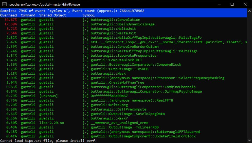
Ok ok I try to do a deeper dive into what’s was going. The optimization test were conducted on the AArch_64 machine named Archie, and the x86_64 machine Xerxes. Both were given an image to process that would result in more than three minutes of processing time, relative to what each machine could handle. Archie used the default bees.png image that comes with the source code distribution, and Xerxes used a 720p image with full background detail.

Default png
Compressed using the default level 3 optimization
Compressed using the fast level optimization

Default png
Compressed using the default level 3 optimization
Compressed using the fast level optimization

Now when I ran perf on each machine per test to see what was going on, and what I saw suggest a SIMD (Single Instruction Multiple Data) approach would likely be the best way to optimize the program.

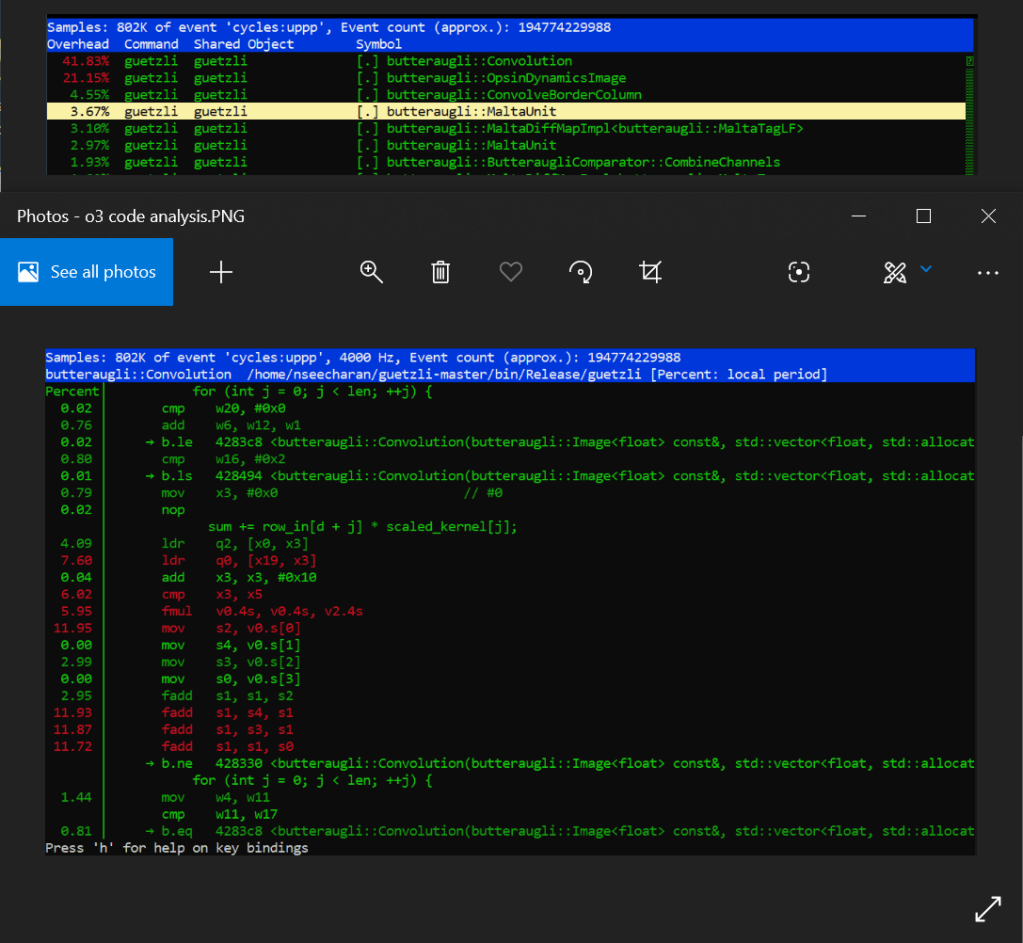
Archie

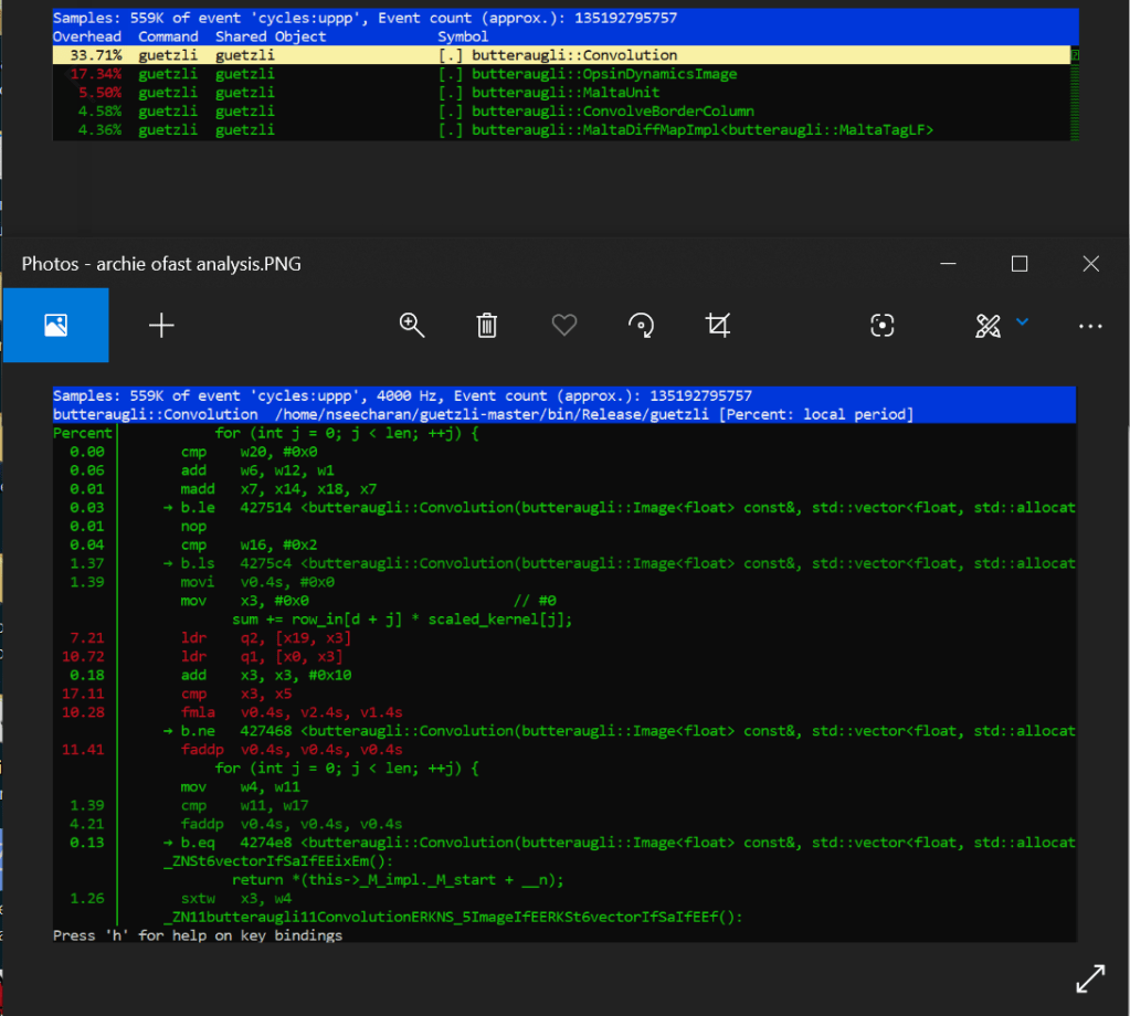
Xerxes

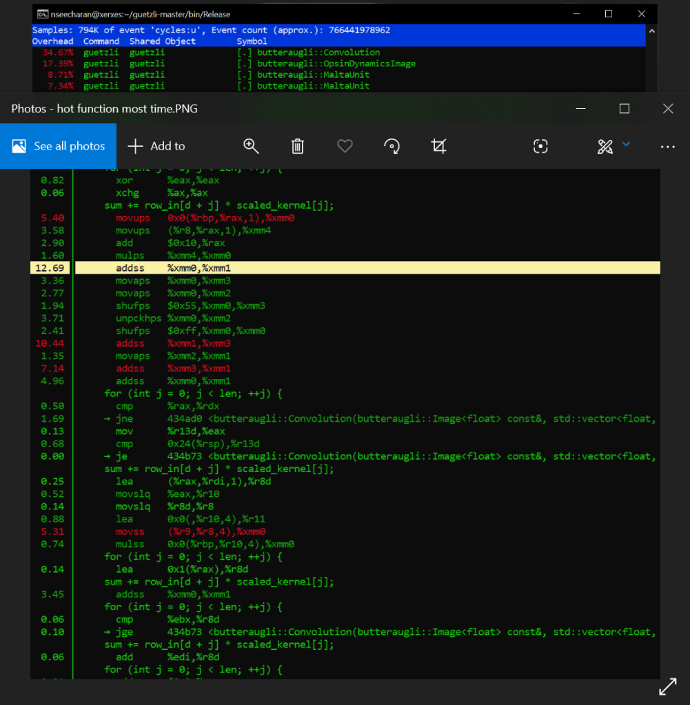
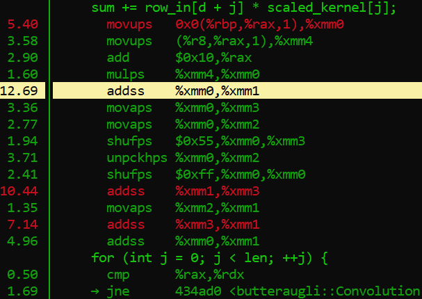
When looking at the perf report for Archie, we see that the default code is employing the use of a series of scalar fadd opcodes to handle the single precision floating point values from what appear to be an array of data. At the very least it’s incrementally adding and storing four separate values, into one final value, which are all loaded into memory with four related move opcodes. Why is this you ask? Well this is likely due to an image being made up of three color channels: Red, Green, Blue, as well as an Alpha channel for transparency, with each channel holding varying levels of “intensity” data; RGBA in short. This is why we see four values, adding to one other value to serve as the sum total. That in mind, when you combine these channels together you get a full color image, with the possibility of semi to full transparency. Now according to the arm documentation on the official website, fadd is part of the SIMD set of processor instructions. Further more, it appears that the four fadd opcodes are adding 32bit wide registers together (denoted with “s”). These observations are important to note, as it may suggest that the program is already optimized appropriately for it’s intended function. However more on that shortly.

Looking at the assembler code sequentially, you can really get a sense that it’s doing a lot of similar tasks one by one. Worse still is that when you combine the processing percentages together for three of the four fadd instructions, you get around 36% of a processing load for the conversion. Certainly this is not the most efficient way to do things*. If only you could make all this work happen in parallel…

Well after optimizing the code with the fast level, it turns out that we can with an add pairwise instruction called faddp (vector variant). To keep it simple, this takes a pool of data, and instead of adding everything sequentially, it breaks the data up into pairs, and adds them together until they all combine into one floating point value. This is extremely useful as it means the processor can store data in memory much faster, even if it is arranged somewhat differently. This speed increase is more evident as there is no longer a need to separate and store (move) the data before adding them all up soon after. This SIMD instruction will just break up the data logically, and store them all at once in a single address that can hold the the length of that data.

Now I have to make another confession. You may have notice that nice boded * two paragraphs ago. I did that because suggesting fadd is not an efficient implementation is a bit unfair. You see, pairwise operations can have a some errors when rounding off values, and if preserving as much detail as possible is your goal, then speed may not be the main focus here. This may be the reason why the developer used optimization level 3 instead of fast, as it relied on a slower but potentially more precise way of processing data.

Well it looks like this a done deal then! Yes, but I would be remiss if I did not at least mention why vadd was likely not used by the compiler. When building code into a piece of software, the compiler tries to translate it to assembler code, that is as efficient as the optimization level allows. In this case, we are only ever working with 32bit length values, so anything larger than that would just be a waste of memory, and overkill of an operation for the task at hand. That in mine, vadd would serve us better when working with data of longer bit lengths. Ok now that’s the final nail in the coffin! Now that much of the logic changes have been established, (not to mention I kind of already did an analysis of the assembler code in stage 2) I’ll try to keep the x86 test on the short side for everyone’s sake haha!

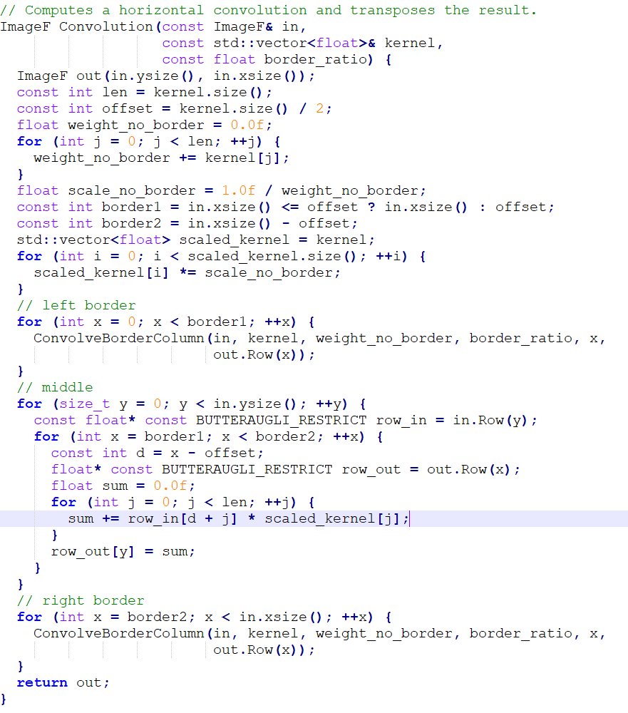
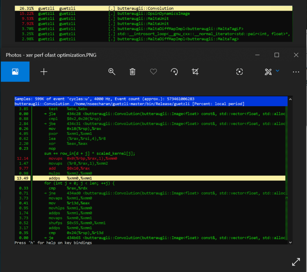
Ok so Xerxes, what are we seeing in the default optimization versus the fast setting for x86_64? Just like the AArch_64 test, there are a lot of similar processes happening one after the other, while also carrying out instruction to store the data in memory in an aligned manner via moveaps. We also see that it is using the unaligned variant moveups to store the two values that represent the “row_in” and scaled_kernel variables of the C++ code. This is of course is just an assumption, but it is based on the on the data we see the mulps opcode using (multiplication for floating point values). There is also shuffling (shufps) and unpacking (unpckhps) of the values just to make this += operation work.

That is quite a bit of work the processor is doing huh?

Well when we look at the fasts solution, we see that the addps SIMD opcode completely eliminates the need to store so many separate values into memory, only to just sum them up soon after. It can work with four packed floating point values which basically covers all four addss right there, basically eliminating more that 20% of processing load from just the adds alone! You also remove the need to do shuffling, unpacking and aligning data in memory. Therefore, significantly less instructions get carried out by the processor, which results in a much faster compression process.

Phew! We got through it and I manged to keep it short…ish. Before I put this thing to bed however, I think I need to mention this programs biggest rival in the form of mozjpeg. Mozilla simply knocked it out of the park here, prioritizing speed over pure accuracy, which to be hones, is not really all that noticeable to begin with unless you magnify the JPEG image by three hundred times. Only then will you see a smoothing effect, as opposed to Guetzli, which tries to replicate, if not preserve the natural noise of an image. Now while I think this is admirable, at the end of the day I tend to side with this bloggers assessment that when it comes to working with images, you want conversions to be quick and small. Now while I personally have not tested mozjpeg myself, I have converted my fair share of images to JPEG back when I was a visual effects artist. That in mind, I can honestly say that anything above a 30 seconds is far too much for the needs of the web, and end users alike. This is especially true when the differences in image quality are not all that perceivable by most people.

So what makes mozjpeg so darn fast?

Well for starters their code is written in C, and also makes use of a lot of assembler code for various processor architectures. Also their focus appears to be towards general purpose use, as oppose to trying to create some kind of lossless JPEG. Overall it extremely well optimized to work well on most machines, while guetzil is written in C++, uses only the O3 optimization, and essentially is a wrapper for the Butteraugli image analysis program developed by Google. In the end I suspect that this was just one of many AI related experiments from google, where some devs were probably trying to see if the Butteraugli algorithm could be used in other ways. Personally I think they should just work on a new image format than trying to reinvent the wheel. Who knows though? One day I may need to eat my own words, if in the end the program gets thoroughly optimize, or if budget computers end up being powerful enough to just brute force through this method of processing images.

Well that’s my two cents! Thank you for sticking with me through this process of optimization, and kind regards to my professor for steering me in the right direction when I had questions.

Bye for now!

Project step 2!

Hello everyone, I’m back to report progress on the second phase of trying to diagnose, and propose optimizations for the image compression software Guetzli. If you recall in the first step, we were conducting benchmark test to see exactly what sort of performance we could get out of the program using some of the stock compiler optimization options. What we discovered was that this program is really really slow! So why is this, and also what part of the program is contributing the most to the slowdown? Well in this stage we shall find out!

Earlier this month our professor introduced us to performance monitoring tools gprof and perf to help us narrow down which program functions were taking the most time. Now between the two methods, gprof is far more through in analyzing a program but this is only possible if the program source code has a configuration script. Why is such a file relevant you ask? Well a configuration script is one way to help build a program from it’s source code. That in mind, the way gprof works is that you incorporate it’s code into the program you are testing. Therefore to accomplish this, you would need to modify that configuration scrip with a simple command in the command line. This is great as you get really accurate data, and can export it so that it displays as a very nice looking diagram.

Unfortunately, the program I am testing did not have this configuration script, so I decided to rely on the perf method instead. The silver lining to this was that I did not necessarily need to recompile my code for it to work. Now while this method is not as accurate as gprof, it still has it’s own merits, as you can not only see the C code, but the assembler code it compiles down to when run. This data can also be exported and viewed in a fairly user friendly manner as well, but only through a Linux command terminal.

Ok enough preamble, get to the results!

What you are seeing is a report that shows which functions of the program were taking up most of the processing time when converting a 720p image. As you can also see, I ran this test on the x86_64 machine Xerxes. I did attempt to use perf on the AArch64 machine Isreal, but perf did not seem to be installed. There were some server issues earlier in the week, so the OS might have been reinstalled. In any case, that’s something I will ask my professor about later in the week. For now though, this data will be enough for our purposes. Looking at the list it is clear that the function “Convolution” takes the most time. This makes sens seeing as convolution is actually a artificial intelligence, and image process algorithm. In the case of artificial intelligence this helps in image recognition, however in our case if I had to guess, this helps to determine where the level of detail in the image can be lowered with minimal to no appreciable difference in quality. It’s probably best you click the link I provided on convolution for more information, as it is very through. Not to mention it may even have solutions for speeding up the algorithm… It’s worth taking a look if nothing else.

For now though, my current goal would be to speed up certain arithmetic operations with the current code, and not do focus too much on a full code rewrite. Getting back to the list here, we can actually look into the code of those functions to see the C code translated assembler code:

This is a portion of the convolution code as represented in this display, here is what he code looks like normally:

Now in the perf report we see that there is an assembler opcode operation that takes up 12.69% of the processing withing this single function. The opcode in question is “addss,” which works in a similar to the assignment operator += in conventional programming, but is specifically reserved for floating point values. Now if you look at the C++ code, you will notice that the variable “sum” is of type float, and has been initialized with a single precision floating point value, denoted with f. This is why assembler is using the addss opcode. Frankly, almost all of those assembler opcodes listed in the picture are reserved for handling floating point values. Crazy huh? Well as we have learned, decimals are very very trik… Impossible to represent literally in binary, so it is understandable that working with values like this would require quite a bit of extra processing from the cpu.

Sigh… Sum why couldn’t you grow up to be a fixed point, life would be a lot easier for you…

Well… Actually, it may be possible to apply a fixed point math approach, and potentially speed up things up as well. I recall my professor demonstrating three different approaches to adjusting the volume of a sound sample. One approach was the slow, but very accurate floating point conversion method, another that used a map of possible volume sample values, and a fixed point math approach, that managed to represent the decimal values without actually needing to do any conversions. All had their strengths and weaknesses, but if memory servers, the fixed point method managed to stay fairly accurate, and was also a bit more quick to execute.

This in mind, how I choose to go about this is still a bit up in the air. Do I just rewrite the loop in C++, or override it with inline assembler? Maybe instead I can rely on SIMD vectorization to help with looping code. In any case, I will have to research a bit more, and soon as stage 3 will need to be delivered by the 18th haha.

Well wish me luck and see you hopefully before the 18th!

Small Update

Hello all, last week I spoke with my professor about my test results and it was determined that I should drop using the computer Archie, and instead use a more powerful one known as Israel. This was decided since the guetzli can potentially use up to six Gigabytes of memory and Archie has only four. Israel on the other hand, has about eight times the memory and would not be overloaded as easily. That in mind, I will be using that computer going forward for the next stages.

Regarding performance, preliminary tests suggest that optimization level 3 and fast, have settings that shorten the overall processing time of 3 minutes and 39.5 seconds by roughly one second. Clearly there is potential here so I look forward to how more specific optimization for the program will run on this computer.

Well see you next time!

Summary of Project Step 1

Hi everyone, considering how long my stage 1 post was, I decide to summarize it for better consumption. For links to the various terminology you can look at the original post here.

For my SPO600 project, chose the image compression program “Guetzli,” because it was command line based, C++ in structure, and took a lot of time to do conversions. I also chose this because ideally I want to optimize the code so that it can run on low powered computers, not unlike the ones found in modern smart phones.

Why smart phones? Well smart phones also serve as a fairly powerful digital camera, capable of taking pictures at very large resolutions. This large resolution is of course, to capture as much detail as possible. That said, most if not all smart phones produce these images in the form of a highly compressed JPEG image. For most casual users this will be enough, however due to the ability to share ones experiences via social media; more and more people show a demand for phones with greater camera capabilities. Now there are already cameras that capture incredibly detailed pictures, however they use file formats that hold 32 bit color information like TARGA, TIFF, and PNG. That is to say, the file format stores color information that can be manipulated accurately, to emulate how one would adjust the exposure of an image. This is possible as each color has a brightness range of 24, with the remaining 8 reserved for transparency. In total 32, and yes that’s where the “32 bit” comes into play.

While there are a few hardware differences between a smart phone camera and a digital camera (namely a lens), the major bottleneck for the former is the file format. When compared to a 32 bit PNG image, a JPEGs color information is only 8 bit. It’s a very limited range and can produce visual inaccuracies, even at their best quality. So why do we use JPEG anyway? Well that is because they hold less data, they take up less storage space. This is a good compromise for devices that have low storage capacity, however 1TB SD cards are no longer in the realm of wishful thinking so storage is moot. Also, as mentioned before consumer demand is ravenous, so it may not be outside the realm of possibility to eventually switch to 32 bit file formats in the near future.

Ok so we now have potentially millions of people creating very large, high quality images, so that they can post it on social media. How can we possibly store all that information? Well it is possible if you have money to spare, but companies like to save, and this is where image compression can help. Imagine if you will, an app of one of these social media platforms, with the capability of compressing the image down to a JPEG, but preserving nearly all the detail of the 32 bit image. This would be very convenient for both users and service providers, if it was quick and effective.

Therefore ladies and gentlemen, my challenge will be to optimize the slow, “Guetzli” program so that it can run quickly on low powered computers like the AArch_64. To accomplish this, I conducted a series of tests, on two computers with that processor, and another with the x86_64 processor. The Aarch_64 computers were call Archie and Charlie, while the x86_64 one was called Xeres. The tests data used consists of the same image scaled to typical HD resolutions, or approximations. The only exception to this was in regards to Archie, the weakest of the three computers, where I used an image that had the dimensions of 444 x 258.

With the resolutions constrained mostly to standard sizes, the processing time was less than the intended target of 4 minutes, however processing time still ranged between 3 minutes and 18 seconds, to 5 minutes and 45 seconds. Given that these were not sub second values I decided to proceed.

The Test

For each computer I use an image resolution that resulted in some cpu load relative to the computer, as well as executing the program using 4 additional optimization settings: o1,o2,o3,ofast. I also ran the program a minimum of twice per each optimization level, unless the results appeared to be an outlier. In all cases this was in situations where the second execution ended up taking longer than the first time, which should not happen if the data is the same. Finally, to mitigate any processor load due to multiple users being logged into the computer, I conducted these test from 11am – 4am.

Archie – 444 x 258

Archie’s performance using it’s stock build settings produced a general processing time of 3 min and 18.6 seconds. When using optimization level 1, the time increased by roughly 0.1 seconds; level 2 showed comparable results but the first execution under this optimization did take roughly 0.15 seconds longer that level 1, and about 0.2 seconds longer than the stock build. Level 3 yielded bizarre results with the first execution matching level 2, but the second execution was faster than even the stock build by about 0.1 seconds. The last level, fast delivered results that were faster than the stock build, but still slower than the second attempt under level 2. One other observations was that the time spent accessing the hardware increased under the fast level. Makes sense as instructions get executed extremely fast in hardware. While this was promising, the speed gains were still negligible.

Charlie – 853 x 480

**Full disclosure, the image used for Charlie was scaled down from a 4k image but it did not result in an exact 720 x 480 image.

For Charlie, the results for the stock build were around 5 min and 42.87 seconds for the first run and 5 min and 42.4 seconds for the second run. When comparing level 1 we see a time of around 5 min and 42.75 seconds. If nothing else it was faster for the first run for the stock build, and maintained a consistent execution time for all but one outlier where it took 2 seconds longer. Level 2 fared worse, adding roughly 1 second to the execution time for both runs. Level 3 was faster than level 2, but averaged around 5 min 42.99 seconds. Fast was overall faster than the other optimizations at around 5 min 42.6 seconds, but still slower than the best time for the stock configuration.

This is it for the AArch_64 series of tests. While there is slightly a bit of potential, I believe more testing and optimizations that override the compiler, may be required to get better performance on AArch_64 hardware.

Xerxes – 1280 x 720

**The 4k image scaled down neatly to the 720 resolution which makes the situation with Charlie more strange.

For Xerxes, the stock test results ranged between 3 min and 24.5 seconds, to 3 min and 19.9 seconds. However with optimization level 1, the program managed to drop around 5 second, resulting in an average of 3 min and 19.5 seconds! Level 2 continued this trend by shedding around 0.2 seconds, but oddly enough, it was the first run under this level that yielded the fastest numbers thus far: 3 min and 19.16 seconds. However interestingly enough, level 3 produced consistently slower results than the first two levels, even adding a whole second to the processing time. Perhaps some of the more unsafe settings in level 3 may have impacted the program in a negative way. The same can not be said for the last setting, as it lived up to it’s name and produced results that were indeed faster than all the other settings, with it’s top result being 3 min and 19.14 seconds. The optimizations for fast is clearly the right direction, however this level does increase the file size so that may also be a factor to consider in the future stages.

Well this was the first stage of my optimization research, I look forward to updating you all in the next project post. See you then!

Spo600 Project Stage 1

Hello everyone, I decided to continue discussing my lab 6 results in a separate post, so instead today I will talk only about my project. Now in the last post I mentioned that I was going to do something related to video, however as another classmate is covering the same topic, I decided to focus on image compression instead.

The open source project I opted to study is Google’s own image compression routine called Guetzli, which is used to convert png images to jpeg, with minimal loss in quality (lossy). What I found interesting about it was not necessarily that it was from Google, or that it even produced good results. No, in fact I was actually interested in why the code execution is quite processor intensive and slow, when compared to other solutions like mozjpeg. I also wanted to see how feasible the compression solution might be on low powered machines with limited memory, similar to a cellphone. That is more in regards to the AArch_64 computers since another computer that will be used, does not really qualify for that, but still might be fun to test on. More on those machines down below.

That in mind, the developer is quite transparent about this fact:

Note: Guetzli uses a large amount of memory. You should provide 300MB of memory per 1MPix of the input image.

Note: Guetzli uses a significant amount of CPU time. You should count on using about 1 minute of CPU per 1 MPix of input image.

Scary stuff, but I was not daunted proceeded to test the code on 3 of the schools servers: “archie”(AArch_64), “charlie”(AArch_64), and “xerxes”(x86_64). Here is a very basic look at some of the specifications for these machines:

archie:
memory 4GB
cpu 0 1GHz 24 cores (don’t let the number of cores fool you, they are slow)
display GeForce GT 710 (may not be a factor in this as everything is done through the command line)

charlie:
memory 8GB
cpu 0 2.4GHz 8 cores, 8 enabled

xerexes:
memory 32GB
cpu 4GHz, 8 cores *2 threads

Just looking at this you can already tell that xerexes is hardly low powered, and will be able to brute force through the code execution. Therefore, I decided to progressively increase image resolution until I achieved a result that took several minutes to complete. In xerexes’ case that limit was a 1080p image, which is considered a 2MP (Megapixel) image, as far as a 16:9 aspect ratio is concerned. For the other machines, I kept the limit at 480p. In regards to compiling optimizations, I used levels 1, 2, 3, and “fast” , in addition to the default which had no specified level. Finally, I performed two executions of the program per test criteria.

That out of the way, here are the initial results with the stock build settings:

archie

$ time ./guetzli bees.png b.jpg
real 3m18.660s
user 3m14.108s
sys 0m3.885s
$ time ./guetzli bees.png b2.jpg
real 3m18.665s
user 3m14.488s
sys 0m3.506s
$ time ./guetzli 480.png 480_t.jpg
real 16m42.537s
user 16m21.184s
sys 0m18.052s
$ time ./guetzli 480.png 480_t2.jpg
real 16m45.095s
user 16m24.027s
sys 0m17.824s

charlie:

$ time ./guetzli bees.png b_c1.jpg
real 1m8.532s
user 1m6.669s
sys 0m1.747s
$
$ time ./guetzli bees.png b_c2.jpg
real 1m8.508s
user 1m6.903s
sys 0m1.497s
$
$ time ./guetzli 480.png 480_c1.jpg
real 5m42.873s
user 5m35.678s
sys 0m6.626s

$ time ./guetzli 480.png 480_c2.jpg
real 5m42.419s
user 5m35.049s
sys 0m6.857s

xerxes

$ time ./guetzli bees.png bx1.jpg
real 0m15.298s
user 0m14.718s
sys 0m0.552s
$ time ./guetzli bees.png bx2.jpg
real 0m15.211s
user 0m14.663s
sys 0m0.518s
$ time ./guetzli 720.png 720x1.jpg
real 3m24.511s
user 3m16.453s
sys 0m7.637s
$ time ./guetzli 720.png 720x2.jpg
real 3m19.899s
user 3m12.027s
sys 0m7.483s
$ time ./guetzli 1080.png 1080x1.jpg
real 7m27.438s
user 7m11.859s
sys 0m14.645s
$ time ./guetzli 1080.png 1080x2.jpg
real 7m28.931s
user 7m13.267s
sys 0m14.730s

All tests started with the image “bees.png,” which was already provided in the source files for testing. It’s not a particularly large file, with a resolution of 444 x 258, but it served as a good baseline for what to expect. That in mind, I opted to use this file most with archie, and would only move up to 480p when there was a noticeable difference in conversion time for the bees image. In the case of charlie, I felt that I could proceed with the 480p image. Likewise with regards to xerxes, I believed working with 720p would be enough, as anything lower would not provide meaningful results.

On to the results:

For archie, the default total execution time hovered around 3 minutes, and 18.6 seconds, where much of the work was being done in software at around 3 minutes and 14 seconds. This is slow to be sure, but what’s even more surprising is that it progressively got slower to execute between levels 1 and 2; adding an extra 0.1, and at worst 0.3 seconds approximately. Level 3 was a bit different in that it was slower than level 1 on the first attempt, but a bit faster than the default compile settings with it’s second attempt; achieving around 3 minutes and 18.5 seconds. When using fast, I actually did 3 tests attempts as the results were peculiar: the first attempt was comparable to the default settings performance at 3 minutes and 18.6 seconds, but the second attempt was closer to the slow performance of levels 1 and 2 at 3 minutes and 18.8 seconds. The third attempt was again comparable to the default settings. One other thing to note was that it when using fast, the time spent accessing the hardware increased. Makes sense as instructions get executed extremely fast in hardware.

Here are the results for archie:

archie

---default---

$ time ./guetzli bees.png b.jpg
real 3m18.660s
user 3m14.108s
sys 0m3.885s
$ time ./guetzli bees.png b2.jpg
real 3m18.665s
user 3m14.488s
sys 0m3.506s

---level 1---

$ time./guetzli bees.png bo1b.jpg
real 3m18.751s
user 3m14.541s
sys 0m3.579s
$ time./guetzli bees.png bo1b.jpg
real 3m18.780s
user 3m13.978s
sys 0m4.186s

---level 2---

$ time./guetzli bees.png bo2a.jpg
real 3m18.919s
user 3m14.145s
sys 0m4.116s
$ time./guetzli bees.png bo2b.jpg
real 3m18.787s
user 3m14.241s
sys 0m3.896s

---level 3---

$ time./guetzli bees.png bo31.jpg
real 3m18.912s
user 3m14.498s
sys 0m3.746s
$ time./guetzli bees.png bo32.jpg
real 3m18.540s
user 3m13.948s
sys 0m3.945s

---fast---

$ time./guetzli bees.png bof1.jpg
real 3m18.612s
user 3m13.916s
sys 0m4.045s
$ time./guetzli bees.png bof2.jpg
real 3m18.846s
user 3m13.784s
sys 0m4.393s
$ time./guetzli bees.png bof3.jpg
real 3m18.640s
user 3m14.023s
sys 0m3.957s

For charlie, the results were mostly similar to archie in that they showed a noticeable amount of slowdown when compared to the default configuration. Two observation however, was that level 2 produced the slowest results, while Level 3 managed to be faster than level 2, but averaged around 5 minutes 42.99 seconds. Now when looking at the fast setting, we begin to see a glimmer of hope as the execution performance for the first test attempt is slightly faster than the default compile configuration. However, the default setting’s second test result were still the fastest overall. This is definitely a start, however I believe more testing and optimizations that override the compiler, may be required to get better performance on AArch_64 hardware.

Here are test results for charlie:

charlie

---default---

$ time ./guetzli 480.png 480_c1.jpg
real 5m42.873s
user 5m35.678s
sys 0m6.626s

$ time ./guetzli 480.png 480_c2.jpg
real 5m42.419s
user 5m35.049s
sys 0m6.857s

---level 1---

$ time ./guetzli 480.png 480_o1a.jpg
real 5m42.741s
user 5m35.375s
sys 0m6.857s
$ time ./guetzli 480.png 480_o1b.jpg
real 5m42.751s
user 5m35.635s
sys 0m6.606s
$ time ./guetzli 480.png 480_o1c.jpg
real 5m44.614s
user 5m37.364s
sys 0m6.706s
$ time ./guetzli 480.png 480_o1d.jpg
real 5m42.441s
user 5m35.278s
sys 0m6.615s

---level 2---

$ time ./guetzli 480.png 480_o2a.jpg
real 5m43.741s
user 5m36.731s
sys 0m6.446s
$ time ./guetzli 480.png 480_o2b.jpg
real 5m43.106s
user 5m34.911s
sys 0m7.654s

---level 3---

$ time ./guetzli 480.png 480_o3a.jpg
real 5m42.989s
user 5m35.897s
sys 0m6.556s
$ time ./guetzli 480.png 480_o3b.jpg
real 5m42.994s
user 5m35.282s
sys 0m7.144s

---fast---

$ time ./guetzli 480.png 480_ofa.jpg
real 5m42.625s
user 5m35.075s
sys 0m7.046s
$ time ./guetzli 480.png 480_ofb.jpg
real 5m42.589s
user 5m35.429s
sys 0m6.647s
$ time ./guetzli 480.png 480_ofc.jpg
real 5m42.818s
user 5m35.515s
sys 0m6.766s

In the case of xerxes, that machine was providing results that I expected:

as the optimizations increased, the faster the program executed.

Now if you recall, the 720p test the two test results ranged between 3 minutes and 24.5 seconds, to 3 minutes and 19.9 seconds. However with optimization level 1, the program managed to drop around 5 second, resulting in an average of 3 minutes and 19.5 seconds! This was a good start but, if you think this will play out like you expect, then you might want to keep reading:

xerxes

---default---

$ time ./guetzli 720.png 720x1.jpg
real 3m24.511s
user 3m16.453s
sys 0m7.637s
$ time ./guetzli 720.png 720x2.jpg
real 3m19.899s
user 3m12.027s
sys 0m7.483s

---level 1---

$ time ./guetzli 720.png 720o1a.jpg
real 3m19.412s
user 3m11.553s
sys 0m7.464s
$ time ./guetzli 720.png 720o1b.jpg
real 3m19.522s
user 3m11.643s
sys 0m7.488s

---level 2---

$ time ./guetzli 720.png 720o2a.jpg
real 3m19.162s
user 3m11.306s
sys 0m7.468s
$ time ./guetzli 720.png 720o2b.jpg
real 3m19.973s
user 3m12.013s
sys 0m7.561s
$ time ./guetzli 720.png 720o2c.jpg
real 3m19.247s
user 3m11.198s
sys 0m7.654s
$ time ./guetzli 720.png 720o2d.jpg
real 3m19.248s
user 3m11.365s
sys 0m7.495s

---level 3---

$ time ./guetzli 720.png 720o3a.jpg
real 3m19.703s
user 3m11.747s
sys 0m7.564s
$ time ./guetzli 720.png 720o3b.jpg
real 3m20.014s
user 3m12.140s
sys 0m7.481s

---fast---

$ time ./guetzli 720.png 720ofa.jpg
real 3m19.145s
user 3m11.188s
sys 0m7.566s
$ time ./guetzli 720.png 720ofb.jpg
real 3m19.255s
user 3m11.308s
sys 0m7.559s

As you can see, setting the optimization levels did improve performance when using levels 1 -2 (level 2 did have one outlier though). However interestingly enough, level 3 produced consistently slower results than the first two levels. Perhaps some of the more unsafe settings in level 3 may have impacted the program in a negative way. The same can not be said for the last setting, as it lived up to it’s name and produced results that were indeed faster than all the other settings. It did however result in a 2 MB increase to the program file size (default settings weigh in at about 4 MB).

Well this was the first stage of my optimization research, I look forward to updating you all in the next project post. See you then!

Baby Steps Into Optimization

Hi everyone, in keeping the momentum from the last post, last week I was part of a group that was tasked in diagnosing potential bottle necks in three programs, running on different computers. Each computer had a different configuration both in processor and memory, and as a result had varying performance times when executing the set of programs. Now what sort of programs were we running you ask? Well they were three different algorithmic solutions for adjusting an audio source’s volume, through multiplication. One approach used floating point conversion (program vol 1), another use a lookup table (program vol2), and the last used a fixed point conversion (program vol3) to adjust the volume of each sound sample it was processing.

So what was the initial predictions at first? Well for me I believed that a lookup table would have been helpful for computers with low processing power, and that computers with more memory would see speed gains as well. That said, unless the lookup table had values for every possible level at 2 degrees of precision minimum, the volume adjustment would likely be not as accurate or smooth. In other words the approach in vol2 would be the least processor intensive, but less accurate. Regarding vol1, my only thought was that processing time would be greater because it was trying to represent decimal numbers (float), with whole numbers (integer) through a conversion. In other word, more accurate, but also more processing intensive. Now in the case of vol3’s fixed point method, I assumed it would be faster than vol1 as there was no conversion, but I had no idea on what the accuracy might be like. That said, I did think it would be slower but more accurate that vol2.

With early predictions out of the way, our group had access to servers hosting five different computer configurations to run our test; 4 AArch64 configurations, and one x86_64 configuration. On each computer we did two pairs of tests: the first pair ran the programs with their algorithms to process the data removed. This gave us a baseline to see what other kinds of stress these programs were putting on computers. The second pair of tests included the algorithms, so that we could see what the full impact of each program was. Afterwards, we could then determine how much of a load the actual processing caused on the computers by subtracting the two test results.

So what was the results? Well for the sake of this post lets observe results from 2 AArch64 configurations, as well as the x86_64. Each of these computers had names assigned to them so I will use these names to refer to each one:

Archie –> The wimpy kid with lot’s of heart
AArch64
4GB memory
1GHz processor with 24 cores
two 32KB L1 cache
256KB L2 cache
4MB L3 cache
GeForce GT 710 graphics card
two hard drives: 1TB, 512GB

Israel –> Fully loaded
AArch64
30GB memory
2GHz processor with 16 cores
32KB L1d cache
48KB L1i cache
1MB L2 cache

Xerxes –> Seemingly unending army of resources
x86_64
32GB memory
4GHz processor with 8 cores but 2 threads per core (virtual cores)*
two 32KB L1 cache
256KB L2 cache
1MB L3 cache

*Makes the processor issue two instructions to each core, effectively doing twice the work, and giving performance close to a process with double the number of cores. This comes with some drawbacks, but this is beyond the scope of this post.

With everyone introduced, I will begin with Archie and continue with the other computers in a follow up post:

Algorithm

Test1

Program	Real	User	Sys
vol1	58.623	56.846	1.614
vol2	64.169	62.095	1.936
vol3	55.731	53.407	2.203

Test2

Program	Real	User	Sys
vol1	58.901	56.958	1.825
vol2	64.345	62.218	1.975
vol3	55.702	53.187	2.405

No Algorithm

Test1

Program	Real	User	Sys
vol1	51.613	49.299	2.214
vol2	51.622	49.17	2.354
vol3	51.388	49.243	2.045

Test2

Program	Real	User	Sys
vol1	51.499	49.347	2.047
vol2	51.731	49.254	2.363
vol3	51.436	49.244	2.096

Dang it Nigel whats with all these weird terms “Real, User, Sys!?”

Haha sorry about that! “Real” refers to the total time the program takes to run. “User” refers to the time taken in user mode, or in other words, when the program is no longer directly accessing the computer hardware, but running through software like an operating system (Windows, OS X, Linux etc). “Sys” is the time the program takes when directly accessing the hardware via kernel mode.

Ok back to the results, at a glance when not using the algorithm, results are reasonably the same with overall execution time being around 51.5 seconds, however take a look at vol2. While execution times were expected to vary as other groups were on the servers as well, vol2’s Sys time seemed somewhat longer than the other two approaches even when no real work was being done. If I recall, we omitted all code related to processing of any data, so really the program should only be loading some data types and the sound sample. This is peculiar but if I had to guess, it may literally have come down to the fact that vol2 had more lines of code:

vol1 = 47
vo2 = 52
vol3 = 46

That in mind, tighter code may result in slightly faster execution of the program. Well what about the numbers for including the algorithm? Looking them over we see some very interesting results. For one, the Sys time is lower for all except vol3, however lets first look at the Real time. Despite taking more time in the kernel, vol3 processes the data much faster than all the other programs. This is even much faster than vol2, which to my surprise, is definitely the slowest method. This of course, completely destroys my initial predictions of the table method being better suited to low powered processors.

Now if looking only at the User phase, much of the processing load is being done here with exception to vol3. For this program to execute it’s math calculations, it uses a low level programming technique called bit shifting, which allows for operations close to the hardware. Therefore, it makes sense that vol3 would take more time in the kernel, as it’s doing it’s bulk of the math there. It should be noted however, that vol1 is no slouch as a solution either. Despite mostly executing in software, it is still fairly quick, and because it runs in the User phase, the data can be salvaged if something fails.

That said with these results, it is clear that optimizing code to take advantage of operations close to hardware, will net considerable performance gains if speed is your goal. If you value safety in the sense of not losing your data, designing code to operate in the user phase effectively is not a bad idea either.

Well these were my initial assumptions, and ultimate discoveries based on the data my group gathered. The next post will talk about the other architectures mentioned, as well as my project. See you then!

SPO Lab 5pt a

Well this was long overdue but I guess better late then never. This past February we were tasked with creating an AArch64 assembler program that would output a message 30 times, while counting upward. Additionally, we needed to suppress (hide) the leading zero for the single digit numbers. We were also tasked with creating a x86-64 version as well.

In higher level languages, this would be a small task, but in assembler there is a lot more setup required to accomplish this result. Further more, despite AArch64 being an assembly language, there are differences in the wording and implementation of opcodes, as well as extra functionality not present in the venerable 6502 assembly language. This was a bit of an extreme comparison given how old 6502 is, however it does illustrate how no two processors may be alike. In the wake of the x86 line of processors however, there has been a some standardization in the assembler language syntax.

Now why do I bring this up you ask? Well as software developers, we may realize that it would be more lucra… I mean, good for the community if the software were available to everyone on various platforms. This provides a challenge however, as hardware differs from device to device, so one can not just transfer the code over and expect it to run. That said, to make the software run, and run well, it requires knowledge of how to optimize the software to cater to the unique specifications of the hardware. This may require one to change how the program is complied, (built), written, or a combination of the two approaches, so that it can operate as expected. In regards to software, this is what we call “porting,” with the optimization aspect being the challenge of this process.

Future posts will touch on this more, but in regards to the lab, as we were dealing with two different types of architecture. Therefore the porting approach we took, was along the lines of writing two versions of the software, to match the instructions that each processor understood.

As the code for the AArch64 version was completed as a group effort, I will not be posting it as part of my git repository, and instead provide it here. Many thanks to Ryan Kortko for basically being the one to write the code as we members provided input:

.text
.globl _start
min = 0
max = 30
_start:
  
  mov x19, min 
  mov x20, 10
loop:
  udiv x22, x19, x20
  msub x23, x20, x22, x19
  add w22, w22, 48 
  add w23, w23, 48 
  mov x0, 1 /* file descriptor: 1 is stdout */ 
  adr x1, msg /* message location (memory address) */ 
  mov x2, len /* message length (bytes) */ 
  cmp w22, 48 
  b.eq printFirst 
  adr x21, msg+6 
  strb w22,[x21]

printFirst:
  adr x21, msg+7
  strb w23,[x21]
  mov x8, 64 /* write is syscall #64 */ 
  svc 0 /* invoke syscall */ 
  add x19, x19, 1 
  cmp x19, max 
  b.ne loop 
  mov x0, 0 /* status -> 0 */ 
  mov x8, 93 /* exit is syscall #93 */ 
  svc 0 /* invoke syscall */

.data
msg: .ascii "Loop: \n"
len= . - msg

Ok so how does this work? Well to begin, I want you to look at the second last line of code where you see:

“Loop: \n”

This is what we will be printing 30 times, however it will display as:

Loop: 0
Loop: 1
.
.
.
Loop:29

Now in our code all we have is “Loop: ” with a new line delimiter at the end. How exactly do we get the number to show up? Well our approach was that we would inject the numbers in the empty spaces after the colon (character positions 6 and 7 to be precise), before outputting the message to the screen. We do this by storing those positions in memory locations x21, and check for whether the next set of numbers to be printed represents a multiple of 10 or not. If it does, print the multiple of 10 in position 6, and then the single digit number in position 7; otherwise print only the single digit number in position 7.

On paper this process sounds straight forward, however assembler does not have typical true or false statements like in the higher languages, so we must exploit some math operations to get the same effect. In this case we can use aspects of division with the opcodes “udiv” and “msub” to get the quotient, and remainder value. You can read more about the opcodes mentioned in this post, here.

There was a time when I called myself an artist…

As the image above illustrates, the 0 above the 5, is the quotient, and the remainder is what’s left when you subtract 6 from 5, in the division operation. In this case it will be 5, as 6 is too large a number to subtract from it. I should also stress that the reason we do not care about long division, is because a processor can not traditionally store a decimal value in binary. That out of the way, this is more than enough to conduct a test to see when the quotient is 0 or not. Take note of the fact that the smaller number (inside number) is being divided by the larger number (outside number). With this setup, any number lower than the outside number, will always result in a quotient that is less than 1, and understood as 0. However once the inside number equals or exceed the outside number, the quotient will stop being 0. Now imagine if the 6 here was a 10, and the 5 was actually a value that started at 1, but would eventually increase and keep being divided by 10. Doing so would result in something similar to this:

0.1,0.2,0.3 …. 0.8,0.9 … and … 1, 1.1, 1.2 …. 2,2.1,2.2
(The numbers in bold are what the processor cares about for this type of division.)

I’m sure you’ve noticed that once the value equals or exceeds 10, the quotient stops begin 0. With this method in place, we can now represent multiples of 10 effectively.

If you recall in the previous lab, I talked about decimal mode, as well as briefly touching on how data is stored in the high byte and low byte. Well in this lab, we can use the high byte value to do some truth testing, to help with formatting the number output. In this case we use “udiv” to get the quotient, which is stored in a high byte, and conversely we use “msub,” to get the remainder, which is stored in the low byte.

In the first loop called “loop:” we store the remainder value in a 32 bit memory address, w23, and the quotient in w22 (32 bit denoted by the w, where as x represents 64 bit). The reason for this is to discard the value’s first half of the 32 bits, as it’s too big to fit in the bit lengh of a character. After that, this is where we do the comparison I mentioned earlier. First we check if the value in w22, equals the character 0. This requires the compare “cmp,” and branch if equal “b.eq,” opcodes. If it does, ignore/skip printing anything in position 6, and first print a value in position 7. We use the opcode “strb” to further discard the excess half of the bits depending on if it is the high byte or low byte. In this way, we can output the characters we need to, and also suppress the bits for the high byte when needed. Without doing so, we would end up displaying the quotient’s 0 values, when outputting the single digit numbers 1-9:

01, 02, 03 … 10,

However the desired output is:

1,2,3 … 10.

I admit this was not a deep dive into the program, as I was not the one who directly wrote it. Also, to not leave it unsaid, I have not even touch on the x86 version, but seeing as how this has become quite a long post, I think I will stop here. The next blog post I will begin talking about my class project topic, specifically what software I will be trying to optimize (video encoding). This should also continue the discussion on porting if only briefly.

Well till the next post!

SPO lab 4 pt 1

Hello all, sorry for the lack of updates, school assignments have been keeping me very busy which is why I have been quiet up till now.

That said, I have some more 6502 assembler goodness to report. Earlier this month the group I was assigned to was tasked with completing two of four assembler coding tasks. We chose to tackle the code that would fill the graphical display depending on the color selected in the text display, and the calculator challenge that required us to write code so that a user could add two number, where each could be a maximum value of 99.

Now I’ll be frank and say that I probably will not get around to finishing the second coding task. That will be something I’ll try to tackle on my own time, as well as figuring out how to make a two player pong game… What I can talk about though is the work I did on the color display. For this particular lab, our professor provided “Rom Routines” for the 6502 emulator we are working with, and they mainly relate to displaying text on the screen. Now you may be asking,

“What the heck is a Rom Routine?”

Well in simple terms, it is per-programmed code which is stored in memory chip, and can be used to complete various operations, as well as add extra functionality to the computer chip’s set of instructions.

That out of the way, what did I do for my program? Well, the main ones I used helped in outputting text to the screen (“CHROUT” aka character output), while using another (PLOT) to get, and set the horizontal / vertical position of the text cursor. You can learn more about all the routines that were available to us here, however I will be focusing on the two I mentioned above.

Now CHAROUT is pretty straightforward, it outputs one character of text. If you iterate through a sequence of characters, and then call this routine, it will output the sequence.

loop:
lda text,y  ;load memory with a text sequence and add 1 via an index (y) to shift to the next character
beq done    ;finish when the index equals the end of the sequence
jsr CHROUT  ;the rom routine that will output the character loaded into memory
iny         ;increment the index/ basically it's like inputting 1+ in a calculator to count upward
bne loop    ;keep looping if the index is not equal to the end of the sequence

Above you see a basic loop using the CHROUT rom routine. Now try to assume that “text” in the code above is pointing to as sequence of characters stored in an area of memory, in this format:
“h”,”e”,”l”,”l”,”o”,00
Each character is a position in this comma separated sequence and so you need to count through this sequence to print the word “hello.” If you’re wondering about the two zeroes at the end, that is to indicate the end of the sequence.

Ok what about PLOT? Well this can be complicated so I’ll try to keep it simple. The PLOT routine requires a bit of setup to get or set the cursor information. You have to do things like manipulating the carry flag in the processor, which will dictate what operation PLOT should carry out… No pun intended. If you are not sure what I mean by carry, basically it’s how we carry over powers of 10 other digits in a number when doing addition. You know right? In addition you sometimes have to write a “1” over a number to show that the value has been passed on to the next power.
1 <— this is a carry since 3 + 9 = 12
23
+ 29
5 2

Ok math lesson over. When you make that carry disappear for the processor, the PLOT routine will set the horizontal and vertical position of the cursor. Once the position has been set, we as programmers can then modify what is outputted at that position. In regards to my program, I wanted to invert the color of the character where the cursor was located. To do this I have to invoke reverse mode to create the desired effect. How I go about this requires that you understand hexadecimal values, and that anything above a value of 127 will result in reverse mode. As long as you understand this you can then create the desired effect by using mathematical operations like Bitwise Or to modify the value. In my code, if you look at the inc_color section, you will see ORA opcode with the hex value of 80. That value in hex is 128, essentially forcing a characters value to be above 127, and reversing the display. In this case I changed the “-” or hex 2d (represents the value of 45) character’s value to hex ad (45 + 128 = 173) to make it display in reverse.

Well that is all for this month, next week I should be able to update you on my next lab assignment using the AArch64 architecture. Please look forward to it!

SPO Lab 3 part 2

Well I took a crack at creating a program to increment a number up to a maximum value of 99. While I did create visuals for the first number, I did not get around to displaying the second number. I did however program a means for both digits to increase in a way that looked like it was counting up to 99. My approach was a bit of a cheat in that I was not actually counting to 99, but instead would only increase each digit independently. The left most digit would increase every 10 button presses, and the right most digit would increase for every button press. I stored values to count these input presses, in two separate addresses: $13 and $14. When you run my program in the 6502 Emulator, if you enable the “monitor” feature, you should see these addresses increasing and decreasing in value accordingly. O’ I should mention that the keys to change the values are the up arrow key and the down arrow key. The assignment stated to use the plus and minus keys, but I used the arrow keys for the sake of ease when testing.

Now I mentioned that I was tracking the numbers independently, however while this approach was adequate, there is a better way. That is of course decimal mode! For the non technical, it is exactly as it sounds in that the values used in a program can be a decimal.

How do they do this? Well a byte consists of 8 bits: 11000010
Now the first four to the left are called the “high byte” and will represent anything left of a decimal. The low bytes are the remaining four to the right, and represent anything right of a decimal. Now I could enable decimal mode, separate the individual values through an anding process using the “AND” opcode. Now you may be wondering what is anding, well if you skipped the hyperlink then the easiest way to explain it is a test of a true or false, but with a bias for false. All maybe or 0.5/0.5 results will always be considered false with this test so only a 1/1 situation will be considered true. For example I am doing an anding operation on 10110011:

00001111
10110011
________
00000011

Now here is the result after the AND. You may have noticed that only 1 and 1 matches remained! Also, in this particular case I we managed to save only the last four values in 10110011. This is how one could separate the value of the low byte. Ok, so what about the high byte? well we could then do a dividing operation with a logical shifting the bits to the to the right so:

10110011
—–>
00001011

This is how we can get the high byte value. Now the great thing about this setup is that you are actually counting properly, and the numbers displayed have an actual computational value. This means you can do standard math operations on them should you choose to implement it. With my cheat method, such a thing would be extremely complicated to do.

Well I believe this was the last of the 6502 assembly labs, which was unfortunate since I now understand the appeal of this chip. Even though it’s assembly language, its pretty straight forward, not to mention that it’s low memory capacity forces you to keep thing simple and not complicate things. I guess also growing up as an NES kid may have something to do with it, as I know have a better appreciation for the amount of effort, and incredible skill game developers of that era had. Getting this chip to do anything is pure wizardry, and I can totally see the magic in it!

That being said, I’ll probably still try to program some things in 6502. As a side not, I kind of feel as though 6502 is one of those things that should be taught before even touching C or C++, since you get a better understanding of how memory is stored and managed in a computer. That’s my humble opinion of course.

Spo Lab 3

Earlier this week I was introduced to more of the programming capabilities of the 6502 processor. We learned how to properly use subroutines, which I was quite happy about as I had run into a problem with my own experiments in lab assignment 2. It was revealed that you would have to put a BRK (break) between the main code that draws graphics and the subroutines to solve the problem. The reason is because a processor’s memory is separated into sections, or “pages.” Some pages are for graphics, and others are for storing program code. These pages are connected and stacked on top each other. This of course means if you are not careful, it would be easy to store graphical information in pages that should only contain programming information. Basically you overwrite your code and potentially exceed the memory for that page.

With this in mind, my subroutine experiment in lab 2 was basically running a second time in a point in memory that was already at the last address of a page, which would cause it to overflow and spill into the other pages (overwrite). In any case, adding the BRK solved my problem.

Two other important concepts were the ability to store pointers in labels, essentially creating a constant variable that could be reused throughout the assembler code. There was also DCB (declare bit), which allows you to store unchanging value at a memory address. This can be handy for defining data that will never need to change, and can allow programmers to generate rudimentary graphical elements like symbols or numbers:

#000
#000
#000
####

In the example above, you see 4 rows with 4 characters per row. This is a 4×4 graphic or “sprite.” If you look carefully you will see a bunch of “#” characters arranged in such a way that it looks kind of like an “L.” I used the # for illustrative purposes but if you replace them with the value “$6”, then you would generate a blue “L” in assembler. If you then put this in a label, you could then conveniently refer to this graphic, and display it where ever you want on the screen. Cool huh?

In the next blog post I will discuss my progress in creating one of the optional programs for lab 3. However regarding Tuesdays group attempt at completing the lab, we had only managed to create the numerical graphics. Outside of that however, we did start to think of the logic of how to increment the numbers up to 99. The remaining challenge was to understand how to implement keyboard input.

In any case, we will see how far I get with my own attempt. See you in the next post!